(Updated 11-Jan-2022; fixed broken links and updated notebook)
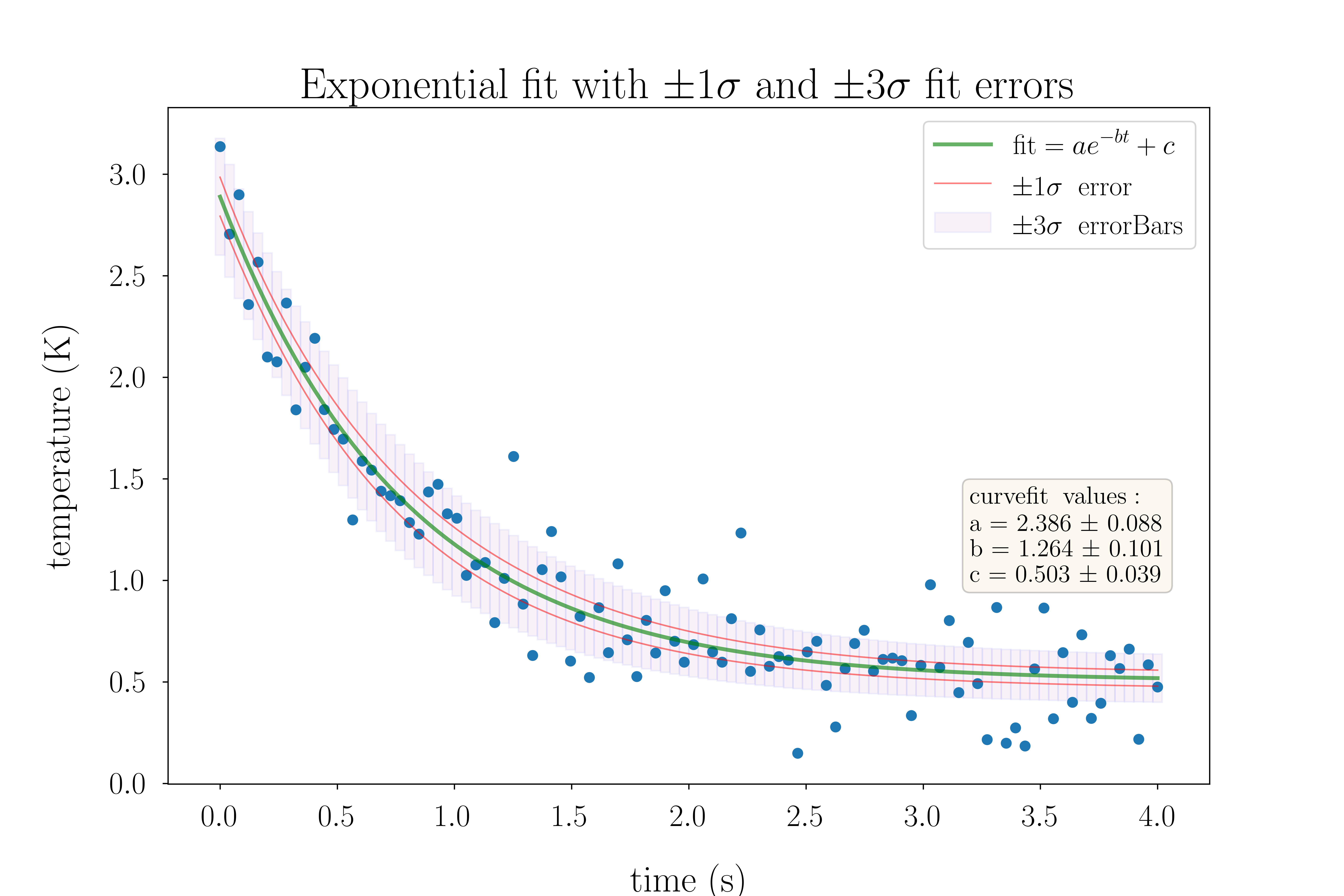
This started out as a way to make sure I understood the numpy array slicing methods, and builds on my previous post about using scipy to fit data. I define a 3 parameter exponential decay
![\[\mathrm{func}(x, a, b, c) = a e^{-b x} + c\]](http://scipyscriptrepo.com/wp/wp-content/ql-cache/quicklatex.com-b52aa73356a92403f8a10767447b6faa_l3.png "Rendered by QuickLaTeX.com")
add some gaussian noise, and then use scipy to get the best fit as well as the covariance matrix. My understanding is that the square root of the diagonal elements gives me the 1  uncertainty on the corresponding fit parameter. So I then use the uncertainties on
  to compute all 8 possible effective parameter values and their corresponding fit arrays.
I then use numpy to find the standard deviation of the 8 different fit values at each x, and use this as the  uncertainty on the fit at a given x. Once I have this array of fit uncertainties, I plot the best fit curve, the fit
 curve, the fit
  curve, and use the matplotlib plot.bar( ) function to plot the
  bars.
bars.
In any case, here is a Jupyter Notebook with some exposition: CurveFitWith1SigmaBand.ipynb
Here is the final plot: (click on link to see .pdf version)
4 Responses to Data fitting with fit uncertainties